If you are looking at a product development and manufacturing team that can seamlessly take your idea to market successfully, look no further. Meet our team today!
Positioning a Linear Servo Motor Using a PID Controller
This article appeared in Electronic Design and has been published here with permission.
Proportional Integral Derivative (PID) control is a common method to regulate the dynamic behaviour of a system. Examples are found in many industrial devices, where they are used for control of temperature, pressure, flow, speed or position, to name a few typical applications.
The theory and mathematics behind PID control have been the subject of much discussion. But how does one apply this math and theory to implement a real device? To demonstrate how to do that, this article will explore a thorough example.
The task of position control will be discussed for the case of a linear servo motor. To begin with, the mathematical function that governs the PID controller’s operation will be presented. We will show how the parts of the function fit together in a practical design. Specifically, we will address considerations for interfacing elements in the electrical circuit in order to accomplish those parts of the PID function for position control, as well as what is involved in implementing the function in the firmware code of a microcontroller that is to do the controlling.
PID Fundamentals
The universal mathematical function which is the basis of any PID control application can be stated as follow:
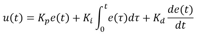
where e(t) is an error value
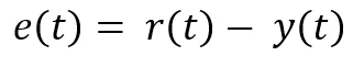
and for the case of position control, r(t) is a set position and y(t) is the current position. A diagram can provide us a much more intuitive understanding of how this math works when applied to our case of a servo motor. Below is the block diagram of a linear servo PID control system.Ok.
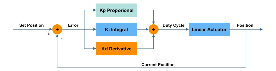
Figure 1 Linear servo PID control system
Some key elements of the system depicted in Figure 1 are a Set Position input (the setpoint, or our target position for the linear actuator), a pulse width modulated (PWM) signal of some Duty Cycle which drives the actuator, and the Current Position of the actuator. These correspond with the quantities r(t), u(t) and y(t) respectively in the mathematical equations.
It is called closed-loop control because a feedback loop relays information about the current state back into the system, allowing it to obtain the difference between this current state and the desired setpoint, which must be corrected. Being specific for our case, Current Position is subtracted from Set Position to obtain the Error (or difference) signal, as shown above. This Error corresponds with the quantity e(t).
And as mentioned at the beginning of the article, PID stands for Proportional, Integral and Derivative. These refer to the three control signals generated for regulating a PID control system’s operation. As indicated in the math and the diagram, the three control signals are produced from the Error signal, are output from the Proportional, Integral and Derivative blocks – labeled also with their respective gains Kp, Ki and Kd – and are combined to produce the Duty Cycle of the PWM signal driving the actuator.
Now that we have described the structure of the system, we want to implement it in firmware. But in order to do this, we need to understand how to interface the linear actuator with the microcontroller – in particular, how the Duty Cycle signal can be obtained from the PID function to drive the actuator, and how the actuator can generate the Current Position signal to feed back to the PID function. We can then explain how to translate the PID function into firmware source code written in the C programming language. Some sample data demonstrating the working implementation will then be presented as the basis for understanding the roles of the three PID control signals and how to tune their performance.
Electrically Interfacing the Linear Actuator
A linear actuator is used for lifting, tilting, pulling or pushing objects. The micro linear actuator we use here consists of a DC servo motor for the actuation part and a potentiometer for the position sensing part. For this unit, the PID controller board needs to output a 12V PWM signal to control motor speed, and use an analog-to-digital converter (ADC) channel to sense the position of the actuator. Accordingly, we should configure two GPIO pins on the microcontroller, one for the PWM and one for the ADC.
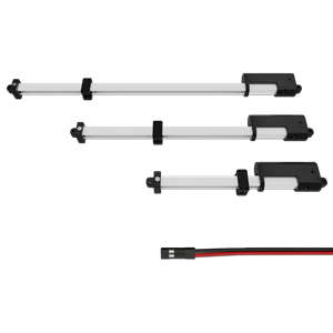
Figure 2 Linear actuators (Source actuonix.com)
The position output of the linear actuator is a resistance value. If the potentiometer is connected between a power rail Vdd and ground as shown in Figure 3, then the resistance at the wiper can be measured as the output of a simple voltage divider. The range and unit of position are changed from 0 ~ 10,000 ohms to 0 ~ Vdd volts, and the ADC converts the voltage to a digital value which is our implementation’s current position y(t). If the ADC’s resolution is 10 bits, this digital value is between 0 and 1023.
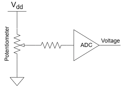
Figure 3 Potentiometer ADC circuit
It is convenient for our controller output u(t) also to be a digital value representing a voltage. However, this controller output drives the linear actuator, which is not expecting a varying voltage as input to control its speed, but a fixed voltage PWM signal with varying duty cycle. Therefore, a conversion is needed. The graphs in Figure 4 below show how voltages from 0 V up to 12 V translate to a 12 V PWM signal with variable-width pulses from 0% to 100% duty cycle. To be strictly correct, voltages above 12 V must also be accounted for, and must translate to a duty cycle of 100%, since the math in no way constrains the controller output to be below 12 V.
As a final remark regarding actuator interfacing, we should emphasize that it is only the nature of the speed control and position sensing features of our chosen device that have guided us to designate u(t) and y(t) both to be (conveniently) voltage quantities in our implementation. These quantities are not otherwise related, and in another application might not even be in the same unit of measurement if the nature of the controlled device’s interfaces were to dictate otherwise.
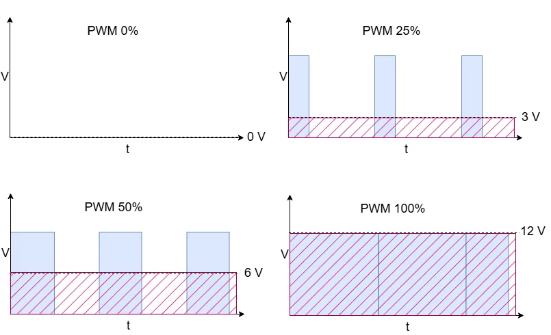
Figure 4 PWM signal graphs
Writing the Firmware
In order for firmware to function as a PID controller, it must determine the error value e(t), evaluate the PID function to adjust the signal u(t) which drives the device, and do this continuously over time. For firmware execution, however, to perform a task in truly a continuous fashion is not a feasible concept. The closest it can come is to repeat – or iterate – the task quickly at short time intervals. If this task is the PID algorithm, then its continuous time math needs to be replaced with a discrete time version, with the following implications:
1. A fixed interval T is designated to be the time between iterations – i.e. their period.
2. Evaluation of the error value e(t) at the moment t in continuous time is replaced with evaluation at iteration n in discrete time – i.e. e(n)=r(n)-y(n), where n = 0, 1, 2, …
3. The continuous time integral of e(t) is replaced by a discrete time summation of e(n)T.
4. The continuous time derivative of e(t) is replaced by the linear slope of e(n) between the previous and the current iteration – i.e. 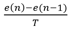
And therefore, the discrete time output signal u(n) evaluated at iteration n can be stated as follows: 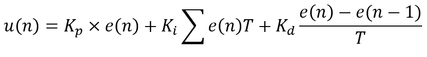
Now we can implement the discrete time PID control function. In the following example C code, variables and constants are given names that closely match the corresponding elements in the mathematical equations. This code can be executed in each iteration of the PID firmware, typically within a timer interrupt configured to trigger every T milliseconds.
 /* Current Error - Proportional term */
 e = r - y;

/* Accumulated Error - Integral term */
 totalError += e;

/* Difference of Error - Derivative term */
 deltaError = e - previousError;

/* PID control */
 u = Kp * e + Ki * (totalError * T) + Kd * (deltaError / T);

/* Also prepare for next iteration – set previous to Current Error */
 previousError = e;
What remains to be done is assign proper values to the PID gains Kp, Ki and Kd so that the system performs correctly when asked to move to a chosen setpoint. We will manually select different values for these gains to investigate their effect on position control, and in so doing, demonstrate a common approach for tuning them. We will also provide some insight into the purpose of each term in the control function.
PID Gain Tuning
There are several criteria for evaluating the performance of the system, including dead time, rise time, overshoot, settling time and steady-state error. While performance expectations should be defined according to these criteria before tuning the PID gains, such expectations depend on the application’s requirements. So for the purpose of this article, it will be sufficient to provide some sense of when various criteria are affected by the adjustment of the different gains.
Each of the gains Kp, Ki and Kd will be tuned separately, and in that order, given a selected setpoint. More specifically, the code will be executed with one of the gains set to a different value for each execution, and the value of r set to 700. As to the relevance of this 700 value, the reader should recall that Current Position is a digital value representing the voltage obtained from the actuator’s potentiometer, and Current Position is now represented by the variable y in our code. The Set Position – represented by the variable r in our code – is a digital value in the same range, which as mentioned previously is between 0 and 1023 if the ADC has 10-bit resolution. A setpoint value of 700 is therefore reasonable, although arbitrary.
a. 5.1 Tuning Kp to get close to the target position
Kp is the proportional gain. The proportional term of the control function compensates for the current error by moving the linear actuator with a signal proportional to this current error. It makes sense that the proportional term is used to get the current position close to the target, since this error is the difference between the actuator’s set position and its current position, and the proportional term makes the control function seek to reduce it to zero.
In this first step of tuning, we set the integral and derivative gains Ki and Kd to zero, and increase the proportional gain Kp until the actuator settles near the target position (700). A proportional gain which is too high will cause oscillation.
The graphs in Figure 5 show how the actuator’s current position changes over time for different values of Kp. We will select Kp = 1, observing that it causes the current position to settle near the target and with the fastest settling time.
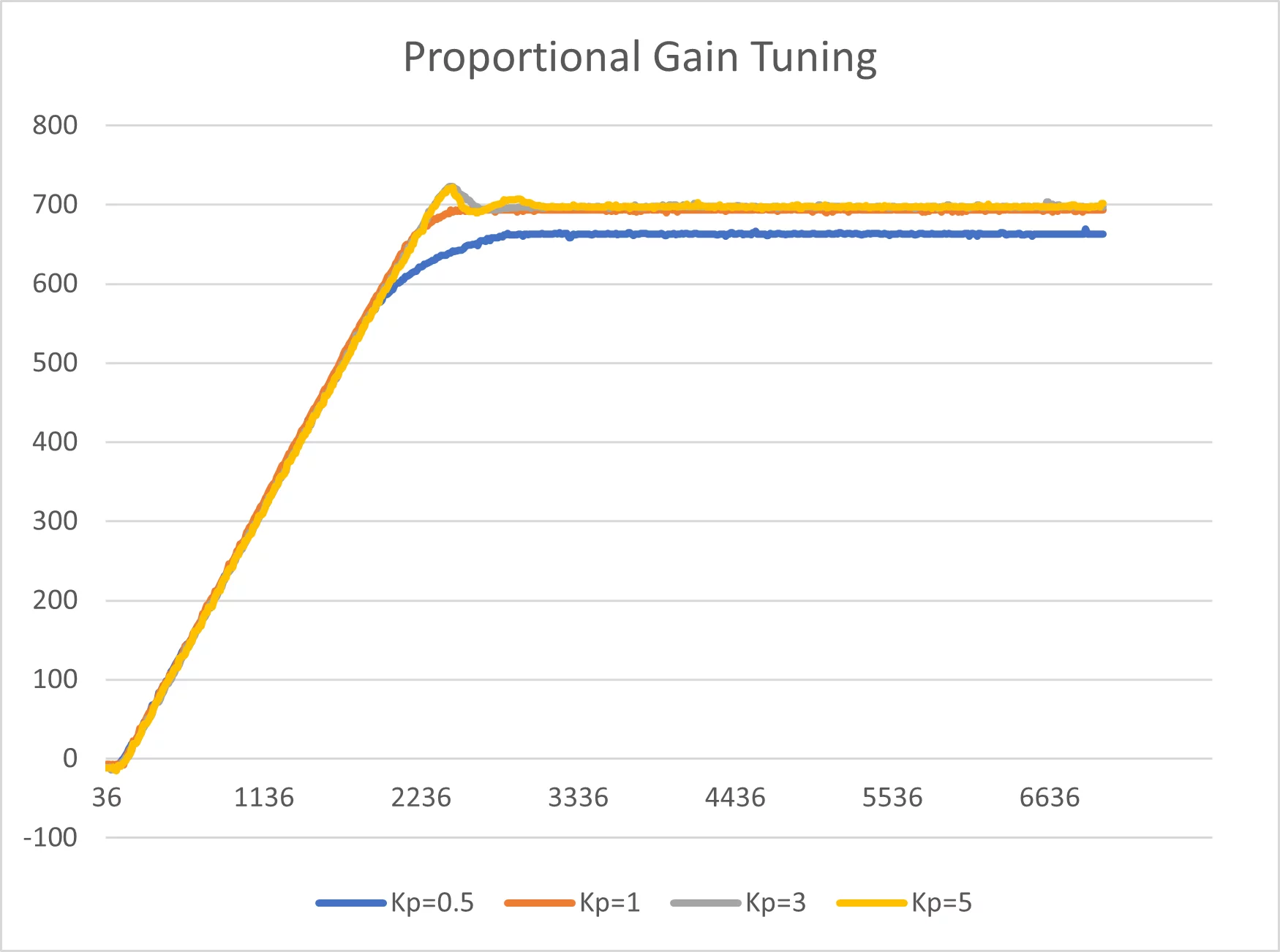
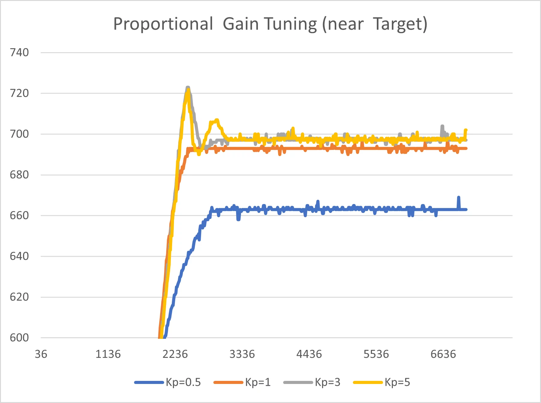
Figure 5 Proportional Gain Tuning
The reader will notice that there is a residual steady-state error, where the final current position is offset from the target setpoint position. This offset is common in the case of a purely Proportional controller, and will be eliminated when the integral gain is tuned in the next step.
b. Tuning Ki to eliminate steady-state error
Ki is the integral gain. The integral term of the control function compensates for the past error by moving the linear actuator with a signal proportional to the amount of this past error which has accumulated over time. It makes sense that the integral term is used to eliminate steady-state error, since this error is a constant offset which grows the integral over time, thus making the control function seek to reduce it to zero.
In this second step of tuning, we keep the proportional gain Kp = 1 selected in the first step, set the derivative gain Kd to zero, and increase the integral gain Ki until the actuator settles much nearer the target position (700) – i.e. until the stead-state error is close to zero.
The graphs in Figure 6 show how the actuator’s current position changes over time for different values of Ki with Kp = 1. The results for Ki = 0.5 may be quite satisfactory for a given set of requirements, and we may elect not to involve a derivative term, in which case the solution would be a Proportional Integral (PI) controller.
Alternatively, however, we may prefer to select Ki= 2, perhaps due to the improved rise time shown in its results. The reader will notice that the better rise time in this case comes at the expense of an overshoot. This overshoot will be eliminated when the derivative gain is tuned in the next step.
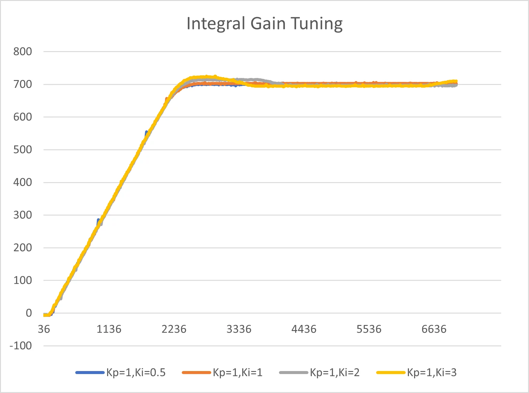
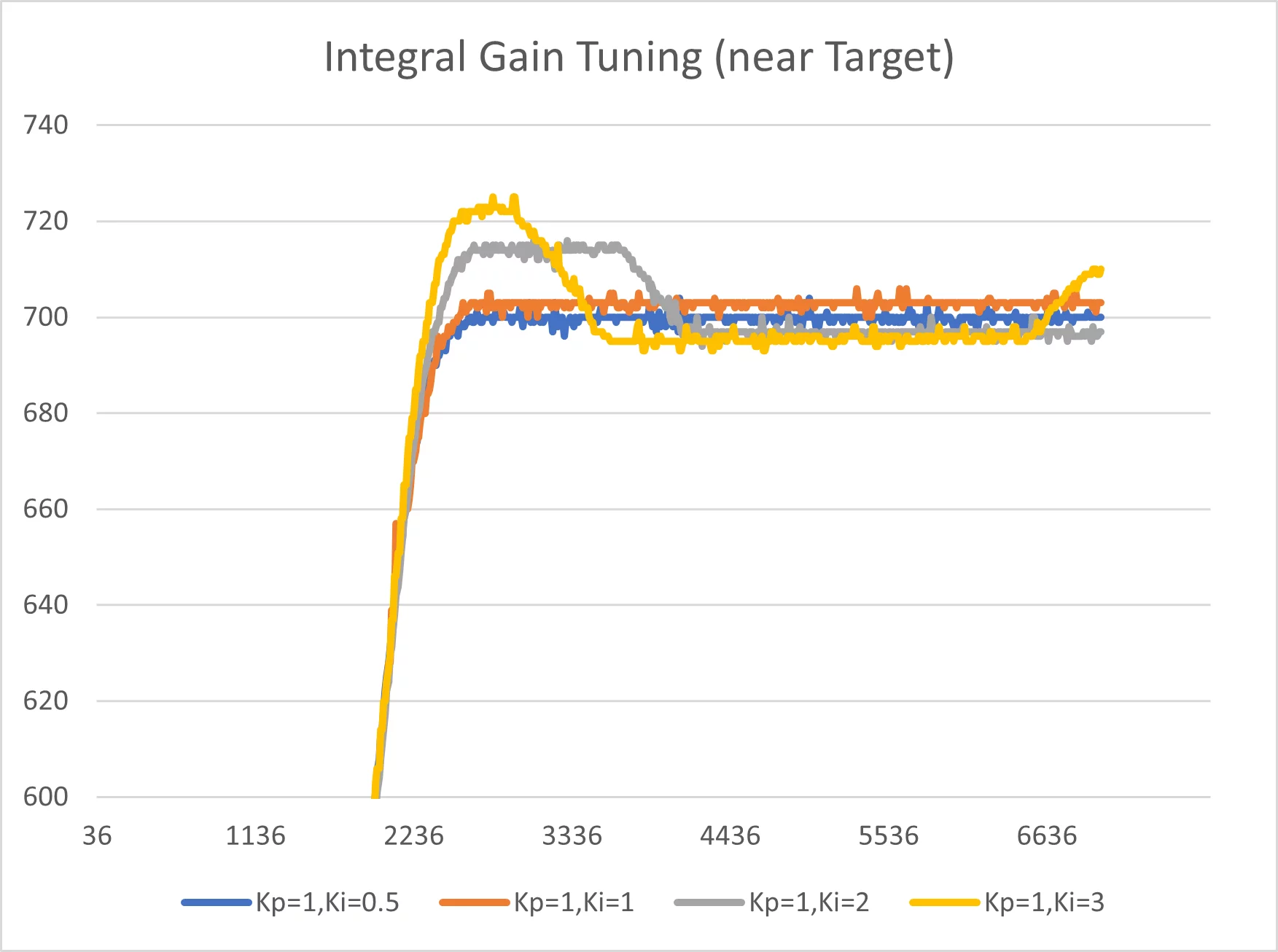
Figure 6 Integral Gain Tuning
c. Tuning Kd to eliminate overshoot
Kd is the derivative gain. The derivative term of the control function compensates for the future (estimated) error by moving the linear actuator with a signal proportional to the amount of this future error as estimated based on the time derivative of the error – i.e. its rate of change. It makes sense that the derivative term is used to eliminate transient effects such as overshoot, which are naturally reflected in the time derivative, thus making the control function seek to reduce them to zero. Improved stability in the presence of disturbances and better settling time are additional related benefits. Note however, that the derivative term can make a control system unstable if the error signal is very noisy.
In this third step of tuning, we keep the proportional and integral gains Kp = 1 and Ki = 2 selected in the first two steps, and increase the derivative gain Kd until the overshoot is eliminated. A derivative gain which is too high will cause oscillation.
The graphs in Figure 7 show how the actuator’s current position changes over time for different values of Kd with Kp = 1 and Ki = 2. We will select Kd = 0.05, observing that it effectively reduces overshoot while maintaining improved rise time.
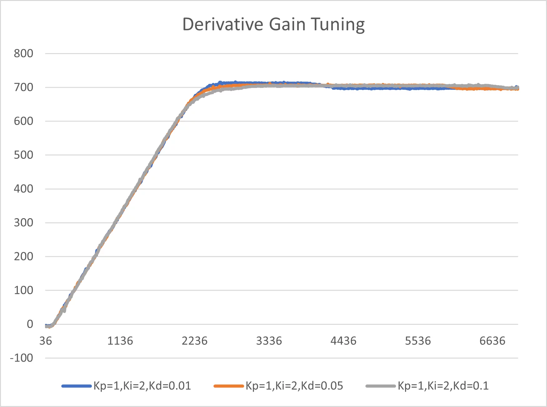
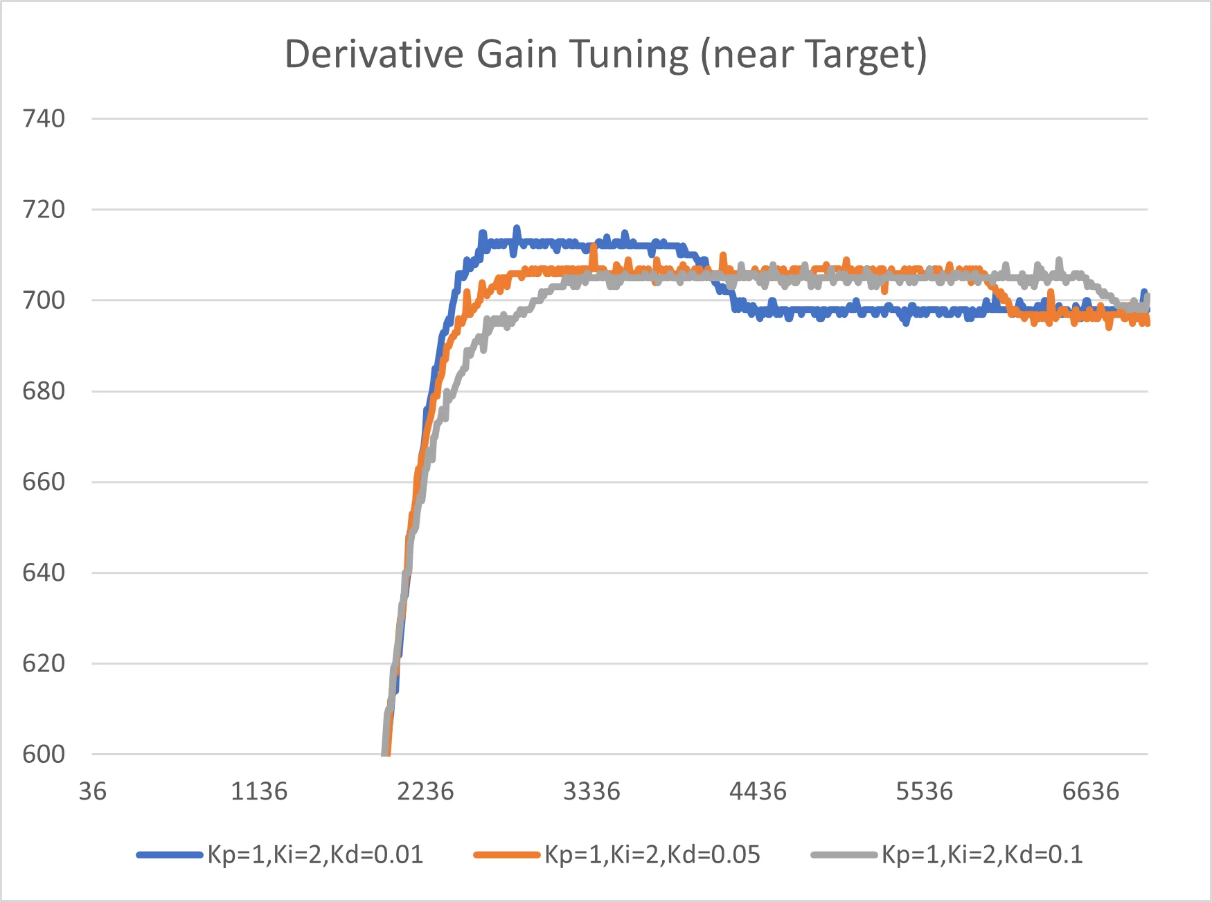
Figure 7 Derivative Gain Tuning
In the version of our controller then, which has all three signals Proportional, Integral and Derivative enabled, we have successfully tuned their gains for proper controller behaviour, and determined that the gain values should be Kp = 1, Ki = 2 and Kd = 0.05.
Conclusion
This article has been about PID control. It explained the mathematics at the heart of a PID controller, and also provided a practical example of how to implement this math to run on a microcontroller. Practical considerations were discussed, about the nature of signals between the microcontroller and a DC servo motor for the purpose of position control. Finally, some data was presented to demonstrate how the Proportional, Integral and Derivative terms of the control function can be manually tuned for proper performance, and to give the reader an idea of the purpose served by each of them in the PID algorithm.
Instead of designing PID control into a custom embedded device, generic off-the-shelf PID controllers are available alternatives in the industrial market – some of which, for example, are based on programmable logic controllers (PLC’s). These may satisfy the needs of many users. However, perhaps not yours if your application requires non-standard functions related to your plant processes. Or has special data communication needs. Or if the generic controller has unneeded features you wish to avoid for a cost-sensitive application. A custom PID controller design is an option in such cases. We are ready to support you with it.
All Blogs